Codebase: https://github.com/msbutler/cs205final
Problem Statement
Climate change has brought about increasingly frequent natural disasters, including flooding, thereby threatening human lives and infrastructure amongst others. Access to accurate and identifiable visual data is extremely instrumental for a directed and efficient relief response. The proliferation of unmanned aerial systems (UAS) with inexpensive sensors has led to a host of high resolution images but the main challenge of analysing these images on a high-frequency and real-time basis with high accuracy still stands.
Therefore, our project aims to construct and train a deep image classifier system that identifies flooded regions from these UAS images. This project requires big compute due to protracted training time required for complex deep Convolutional Neural Networks (CNNs), as well as the need for more iterations without using a pre-trained model. Big data techniques are also employed to more effectively manage numerous large high-definition images. Hence, we deploy the model for fast, highly parallelizable classification on Amazon Web Services (AWS).
Existing Work
Several studies in recent years have explored image classification for disaster relief. Gebrehiwot et al. (2019) developed a deep CNN for flood mapping based on UAV data (similar to our dataset).[1] Gebrehiwot reported that it took about 26 hours for cross validation using a single GPU (NVIDIA Quadro M4000). Sarker et al. (2019) developed a supervised CNN for flood mapping based on satellite images.[2] They used a High Performance Computing (HPC) server to train their model rather than a GPU and reported a training time of 24 hours. A more recent study, Hashemi-Beni and Gebrehiwot (2021), also developed a CNN for flood labeling of images, but did not report the infrastructure used for training the model or the required training time.[3]
Instead of a fully-supervised approach as with the studies described above, we focused on building a semi-supervised model because real-world datasets are predominantly unlabelled. Our semi-supervised model is a convolutional neural network (CNN) that learns from both labeled and unlabeled images, therefore requiring a custom loss function and various data augmentations for implementation. Instead of transferring and applying a pre-trained model, we built our CNN from scratch, adapting and simplifying key components from Google’s MixMatch and FixMatch algorithms.[4][5] We elaborate on the specifics of our algorithm in the following section.
Additionally, it is worth noting that this work can be easily extended to other natural disasters like wildfires and debris from earthquakes. We hope this work contributes to the increasingly numerous humanitarian applications of machine learning with big compute and big data.
Model and Data
Model
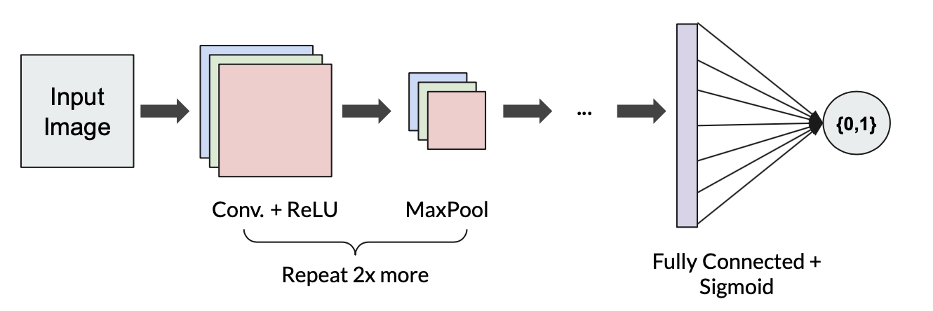
We developed a custom semi-supervised CNN for image classification. The architecture used first consists of 3 convolutional layers with ReLU activation function, batch normalization and max-pooling. The first convolutional layer has a 25 by 25 kernel size and stride length of 10, which is intentionally made relatively larger than the following layers in order to capture broader trends and patterns of the original image. The number of channels increase from 3 (original RGB) to 16. The second and third convolutional layers have a 5 by 5 kernel size and stride length of 2. The second layer maintains the same number of channels while the third layer increases to 32 channels. All convolutional layers have a max-pooling kernel size of 2 by 2 and batch normalization is employed in each layer to tackle the issue of internal covariate shift when the distribution of each layer’s inputs changes during training due to back-propagated parameter updates. Thereafter, the output of the third convolutional layer is flattened and passed to a fully connected layer with an intermediate output size of 64 before a ReLU activation function. Finally, the last layer is another fully connected layer with the final output size of 1 before a Sigmoid activation function, pushing the classification to be boolean corresponding to either a non-flooded or flooded image. This architecture is illustrated in Figure 1 below.
Figure 1: CNN Architecture
During training, we use the architecture described above to classify both labeled and unlabeled images as flooded (1) or nonflooded (0). For labeled images, we want the model to produce predictions that match the ground-truth labels, so we penalize the loss function when predictions do not match the true labels. With unlabeled images, we want the model to assign photos with similar features to the same class. Therefore, we augment each unlabeled image several times and penalize the model for producing different predictions across augmentations of the same image. Augmentations may include rotations, translations, reflections, or noise additions to the original photos. For consistency between the labeled and unlabeled training data, a single augmented version of each labeled photo is used in lieu of the original image.
The training process for a single mini-batch within an epoch is illustrated in Figure 2. We perform a forward pass on the augmented version of each labeled photo and the k augmentations of each unlabeled photo within the batch. For the unlabeled images, a “guess” at the true label is produced by taking the mean of the model predictions for the k augmentations of the same image. Model predictions are then evaluated using cross entropy with the true label (for the labeled data) or the L_2 loss with the guess label (for the unlabeled data). Total loss for the batch is the sum of the labeled loss with the unlabeled loss, where the unlabeled loss is weighted by a constant.
For training, we use the Adam optimizer with a learning rate of 0.001 and 500 epochs.
Figure 2: Outline of Model Training for One Batch/Epoch

Data
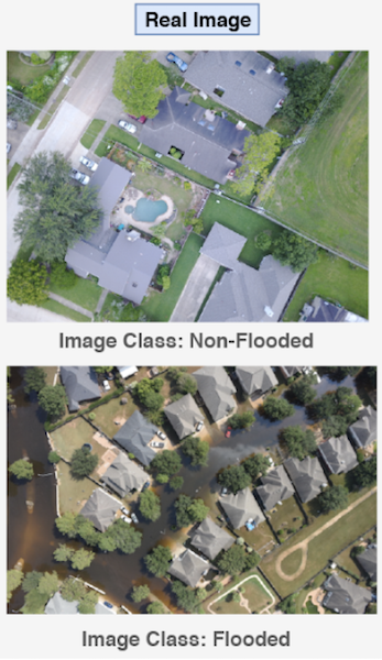
The dataset used comes from the Floodnet Challenge [6], with approximately 2,300 quadcopter or drone images of land from post-Hurricane Harvey. The data is segmented into 60% training, 20% validation and 20% testing sets. Of the training set, 25% is labeled (approximately 400 out of 1,400 images). Examples of a non-flooded and flooded image are shown in Figure 3. These images are of high resolution, 3000 by 4000 pixels, and hence are reduced to 750 by 1000 pixels for more efficient training and memory management.
Figure 3: Example Images for Classification
Our data set consists of 51 labelled flooded images, 347 labelled unflooded images, and 398 unlabelled data images. We used 80% from each subset for training.
Parallel Application, Programming Models, Platform and Infrastructure
Training convolutional neural networks is highly computationally intensive due to the many intermediate calculations required at each point of the architecture. In our situation, this issue is exacerbated by the high quality resolution of our images, which inherently increases the problem size at every intermediate step. Fortunately, matrix multiplication, convolutions, and pooling are all highly parallelizable tasks, and for this reason we relied on accelerated computing with a GPU to speed up the training and evaluation process for our model. This constitutes procedure-level parallelization as we are parallelizing regions of code within a task and thus falls in the external, fine-grained domain of Big Compute.
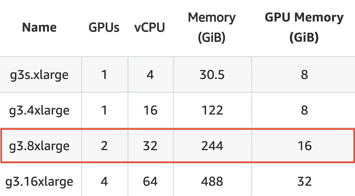
We evaluate performance by training our model on an AWS GPU. Specifically, we use a g3.8xlarge instance with Ubuntu 18.04 and the AWS Deep Learning AMI which pre-configures commonly used machine learning packages into different virtual environments. Table 1 includes additional details about the g3.8xlarge configuration. Python (specifically Tensorflow) encodes our CNN and controls the hardware. Certain operations in Tensorflow (i.e., Matmul for matrix multiplication) include both CPU and a GPU implmentations “under the hood”. If running code on a GPU, Tensorflow automatically prioritizes the GPU implementation of the operation. We control the number of GPUs visible to CUDA (and therefore, Tensorflow) by setting the enviornment variable CUDA_VISIBLE_DEVICES to the desired GPU IDs using the os package.
Table 1: GPU Configuration Details
Note: AWS unfortunately did not grant us a limit increase needed to use the next largest g3.16 instance with four GPUs (we follwed up but still have not heard back from their support).
We have also initially experimented with storing all the images on a AWS S3 bucket but transitioned to downsizing the image resolution and storing it on GitHub due to GPU memory optimization as will be discussed in later sections.
Software Design
Codebase: https://github.com/msbutler/cs205final
As mentioned above, our model is built in Python primarily using tensorflow. We also rely on the os package for reading in data; skimage, random, and PIL for image analysis; numpy for additional data analysis; and matplotlib for plotting our results. Each of these packages comes pre-installed with the AWS Deep Learning AMI. Replication information for producing the same environment with the same package versions used in our tests is included in the Replication.md instructions file on the Github (see Codebase link above).
Our code is structured as follows:
Train/: folder with subdirectories for labeled and unlabeled training dataFigures/: folder containing results from performance tests_old/: folder containing out-of-date versions of filesarchitecture.py: defines CNN architectureconfig.py: configures data parameters (i.e., image resize dimensions)run.py: trains one instance of the supervised or semisupervised modelsemisupervised.py: specifies training methodology for the semisupervised modelsupervised.py: specifies training methodology for the fully supervised modelstrong_scaling.py: script for running strong scaling performance tests (see next section for additional information)weak_scaling.py: script for running weak scaling performance tests (see next section for additional information)utils.py: contains functions for image analysis and developing training/testing sets
Performance Evaluation
We have conducted 2 broad tests to evaluate both weak and strong scaling for our deep classifier. Firstly, weak scaling is tested by increasing the training and testing data as a proxy of the problem increasing proportionally to the number of processors or processing power. Using a g3.8xlarge instance with 2 GPUs, both supervised and semi-supervised versions of the classifier are trained over 5 iterations to generate average training times for 25%, 50%, 75% and 100% of the dataset (both labeled and unlabeled). Secondly, strong scaling is tested by training the algorithm on the full dataset and varying the number of GPUs used on a g3.8xlarge instance by having Tensorflow interface with CUDA, setting CUDA_VISIBLE_DEVICES to different lists of GPU devices as mentioned in earlier sections. Computational times from strong scaling experiments will indicate the speedup of increasing number of processors while fixing the problem size.
Several optimizations were conducted for the parallelization process, including reducing the image resolution size and varying the optimal batch size to fit within the GPU memory as training on the original high-definition images led to various memory issues on the GPU. Nevertheless, there are numerous overheads when training on the GPU and hence, the theoretical speed-up or perfect scaling where computational time decreases linearly with lower training data or generally decreases with more GPUs is not expected. The main overhead for GPU-accelerated computing is the data transfer between the CPU and GPU, where most matrix multiplications and convolutions are conducted within the GPUs. Moreover, it is noteworthy that GPU acceleration is most effective for data parallelization which is suitable in our implementation of weak scaling but is not optimal for speeding up more complex or deeper neural network architectures.
Discussion
Firstly, we note that time to convergence is significantly higher when not using a pre-trained model, as described in the aforementioned sections. Based on the current architecture, the model for both the fully-supervised and semi-supervised approaches have yet to converge with mediocre training and testing accuracies after 1000 iterations, taking more than 3h on a g3.8xlarge instance, especially since most deep classifiers require thousands of iterations for convergence from scratch. We have also experimented with a more balanced dataset by restricting the number of labeled flooded and non-flooded images to be the same. Notably, we did achieve significant results on the fully-supervised model with a more simplified architecture (3 convolutional layers with kernel size of 5 by 5 and reducing the number of channels along the layers) where testing accuracy reaches a peak of around 80% after 200 iterations on a balanced dataset with baseline random accuracy of 50%.
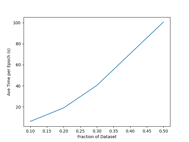
Secondly, the weak scaling experiments for both fully and semi-supervised models corroborate the hypothesis that computational time increases with the data size for both training and testing as shown in Figures 4 and 5 below where the average epoch time (across 5 epochs) is plotted against the fraction of dataset used for training and testing. The fraction of dataset used for the semi-supervised model is half (10%, 20%, 30%, 50% of total dataset) of that used by the fully-supervised version (25%, 50%, 75%, 100% of total dataset) for computational time experiment purposes since the number of unlabeled images are more than the labeled images.
Figure 4: Weak Scaling for Fully-Supervised Model
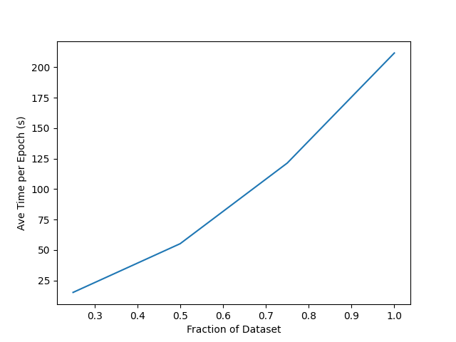
Figure 5: Weak Scaling for Semi-Supervised Model
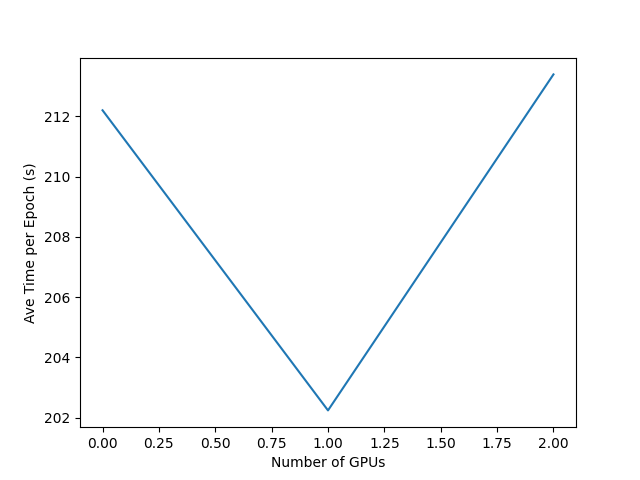
Thirdly, the strong scaling experiments indicated that the theoretical speed-ups were clearly not achieved, due to significant overheads from GPU-CPU communication amongst others. The average epoch time against the number of GPUs used for the fully and semi-supervised models are shown in Figures 6 and 7 below. It is observed that using 1 GPU leads to lower average epoch time when using no GPUs, indicating that GPU acceleration speed-up outweighs the overheads. However, increasing to 2 GPUs resulted in higher average epoch time, with the semi-supervised version exceeding the time without GPUs. This could be due to better optimization in the no GPU case where tensorflow could have better leveraged the 32 vCPUs, thereby not optimally representing a baseline version without GPU. Another potential explanation to the smaller speed-up when using 1 GPU is due to the experiments only averaging across 5 epochs. The first initial epoch requires significantly more time for data transfer and optimization when using GPUs, therefore indicating that averaging over more epochs may result in higher speed-ups when using GPUs compared to the no-GPU scenario.
Figure 6: Strong Scaling for Fully-Supervised Model
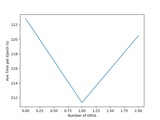
Figure 7: Strong Scaling for Semi-Supervised Model
Conclusion and Future Work
In conclusion, we have successfully implemented a deep image classifier for flood disaster management using both a fully-supervised approach and a semi-supervised model. We have also gleaned insightful observations on the various mechanisms involved in Tensorflow’s interface and interactions with accelerated GPU computing. Weak scaling is corroborated where computational times are higher along with increasing training and testing datasets. On the other hand, the results from strong scaling are different from the theoretical expectations due to significant GPU-CPU communication overheads and averaging over a small number of epochs.
Future work entails leveraging Tensorboard for better insight into GPU analysis in terms of time spent on GPU computations, GPU-CPU communications and potentially better optimizing the allocation of computations to multiple GPUs. Moreover, it would also be worth exploring different CNN architectures or parallelizing deployment of pre-trained models for better model convergence.
Citations
[1] Asmamaw Gebrehiwot et al. “Deep convolutional neural network for flood extent mappingusing unmanned aerial vehicles data”. In: Sensors 19.7 (2019), p. 1486.
[2] Chandrama Sarker et al. “Flood Mapping with Convolutional Neural Networks Using Spatio-Contextual Pixel Information”. In: Remote Sens. 11, 2331 (2019).
[3] Leila Hashemi-Beni & Asmamaw Gebrehiwot. “Flood Extent Mapping: An Integrated Method Using Deep Learning and Region Growing Using UAV Optical Data”. In: IEEE Journal of Selected Topics in Applied Earth Observations and Remote Sensing 14 (2021), p. 2127-2135.
[4] David Berthelot et al. “Mixmatch: A holistic approach to semi-supervised learning”. In: arXivpreprint arXiv:1905.02249 (2019).
[5] Kihyuk Sohn et al. “Fixmatch: Simplifying semi-supervised learning with consistency andconfidence”. In: arXiv preprint arXiv:2001.07685 (2020).
[6] IEEE Earth Vision 2021 Floodnet Challenge. http://www.classic.grss- ieee.org/earthvision2021/challenge.html. Accessed: 2021-04-01.